Adaptive Mesh Refinement for Singular Current Sheets in Incompressible Magnetohydrodynamic Flows
HOLGER FRIEDEL, RAINER GRAUER, AND CHRISTIANE MARLIANI
Institut für Theoretische Physik I
Heinrich-Heine-Universität Düsseldorf
D-40225 Düsseldorf, Germany
The formation of current sheets in ideal incompressible magnetohydrodynamic flows in two dimensions is studied numerically using the technique of adaptive mesh refinement. The growth of current density is in agreement with simple scaling assumptions. As expected, adaptive mesh refinement shows to be very efficient for studying singular structures compared to non-adaptive treatments.
The formation of singularities in hydro- and magnetohydrodynamic flows is still a controversial issue in the mathematics and physics community. Since mathematically only very little is known [1], one has to rely on numerical simulations. Even in very elaborate numerical experiments (see Bell and Marcus [2], Kerr [3]) non-adaptive treatment is limited very soon by the computer memory available, resulting in a resolution of less than 512 grid points in each spatial direction. Since the singular structures like tubes and sheets are not space filling, adaptive mesh codes seem to be the right choice for studying these problems, as has been done by Pumir and Siggia[4,5]. Unfortunately, the methods used in [4,5] could only refine the region around a singular point which lead in [4] to a substantial loss of energy. Of course, it is desired to refine all regions where the numerical resolution is insufficient. Modern adaptive mesh refinement algorithms, as introduced by Berger and Colella [6] and Bell et al. [7], do not possess the above limitations and are good candidates for studying singularity formation even in incompressible systems.
In this paper, we investigate the formation of singular current sheets
described by the ideal incompressible magnetohydrodynamic equations (MHD
equations) in two dimensions for the time evolution of the velocity field
![]() and magnetic field
and magnetic field
![]() . Using Elsässer
variables
. Using Elsässer
variables ![]() ,
the MHD equations take the symmetric form
,
the MHD equations take the symmetric form
The equations (1) are integrated in a
periodic quadratic box of length ![]() using
adaptive mesh refinement with rectangular grids self-adjusting to the flow.
In each rectangular grid, a projection method is used where the time-stepping
is performed in a second order upwind manner [8,9,10].
For the projection step, we need the vorticities
using
adaptive mesh refinement with rectangular grids self-adjusting to the flow.
In each rectangular grid, a projection method is used where the time-stepping
is performed in a second order upwind manner [8,9,10].
For the projection step, we need the vorticities ![]() and
potentials
and
potentials ![]() which
are related by
which
are related by ![]() .
.
The outline of the paper is as follows. In the next section, the adaptive mesh refinement algorithm is introduced. Then, we discuss the numerical results and compare the growth of current density with the prediction of Sulem et al. [11]. Finally, we conclude that adaptive mesh refinement is an ideal tool for studying singular structures and should be pursued further to study three dimensional problems as the finite time blow up in the incompressible Euler equations.
The main idea of adaptive mesh refinement is simple. One starts with a grid of given resolution and integrates the partial differential equation as usual. As soon as some criterion is fulfilled, this initial grid is refined. This is done by marking all critical grid points where the discretization error exceeds a prescribed value. Then new grids with finer resolution and timestep are generated which cover all these critical points. These grids belonging to the next level are then filled with interpolated data from the first level. Then, one integrates both levels until the resolution again becomes insufficient. Now the critical points are collected over all grids of the actual level being refined. Filling the new grids with data is achieved by first taking data from the previous level and, if existing, data from former grids of the same resolution. This process is repeated recursively. In addition, to communicate the boundary conditions, each grid needs information about its parent grids and its neighbors. As one can see already, adaptive mesh refinement requires the management of lists of levels, critical points, grids, parent grids and neighbors. Therefore, we programmed the handling of those structures in C++ whereas the numerically expensive integrations are done in fortran. In order to encourage the reader to use adaptive mesh refinement we describe the above outline in more detail in the next paragraphs.
To deal with all the different lists we defined templated list classes and iterators which can be used for all classes representing levels, grids, critical points, parents and neighbors.
The integrator used for all grids is based on a projection method combined with second order upwinding. This scheme motivated by Bell et al. [8] was previously applied to incompressible magnetohydrodynamic flows in two dimensions [10]. It is clear, that the equations under consideration can be easily exchanged by other ones using an explicit algorithm since the structures needed for adaptive mesh refinement and the integrator are independent of each other.
The timestep on a given level is advanced as illustrated by the following piece of pseudo-code.
procedure integrate level
do singlestep on level
better boundary on level
solve poisson equation on level
if next level exists, then
default boundary on next level
do r times
integrate next level
update of level
check criterion on level
The criterion for refinement is adapted to the problem of current sheet formation. The global maximum of vorticity and current density is calculated and compared to the values when the last refinement was done. Regridding is initiated, if the ratio of those maxima exceeds a prescribed value which is equal to the refinement factor r due to the scaling symmetry of the MHD equations (1). The result of regridding is a new list of levels starting below the actual level. This new list replaces the old one, which is then deleted.
The logical structure of the regridding procedure is shown in the subsequent pseudo-code.
procedure regridding level
for all grids on level
mark critical points and append them to a list
cover the critical points with rectangles (saw up)
nesting rectangles into their parents and
assign parents and neighbors
fill the new rectangles with default data
calculate global maxima for comparison in the procedure check
if old level of same resolution existed before regridding, then
better data on new level from old level
solve poisson equation on new level
if finer level existed before regridding, then
regridding of new level
else
assign global maxima from old level
else
solve poisson equation on new level
The procedure regridding starts
with a loop over all grids of level to collect the critical points.
Therefore, we calculate at each grid point the difference between the convection
terms ![]() on the
actual level and the next coarser one and if this difference exceeds a
prescribed threshold
on the
actual level and the next coarser one and if this difference exceeds a
prescribed threshold ![]() ,
we append this point and a surrounding rectangle of given size to the list
of critical points. In the procedure saw up
these critical points are covered with rectangles. The procedure
nesting guarantees that they are properly
nested into grids of the previous level allowing for more than one parent
grid. At the same time, parent and neighbor grids are assigned to each
new rectangle. Since these procedures are the most complex ones, they will
be discussed in detail in the next subsections.
,
we append this point and a surrounding rectangle of given size to the list
of critical points. In the procedure saw up
these critical points are covered with rectangles. The procedure
nesting guarantees that they are properly
nested into grids of the previous level allowing for more than one parent
grid. At the same time, parent and neighbor grids are assigned to each
new rectangle. Since these procedures are the most complex ones, they will
be discussed in detail in the next subsections.
Now as each rectangle has information about his parents, the new rectangles
are filled with spatially interpolated data in default
data. To avoid discontinuities, interpolation is done on the
fields containing the highest derivatives, namely ![]() .
In order to supply boundary conditions for the solution of the Poisson
equations, data for the potentials
.
In order to supply boundary conditions for the solution of the Poisson
equations, data for the potentials ![]() on
the outermost boundary are assigned as well. Afterwards, global maxima
needed in the procedure check are calculated.
on
the outermost boundary are assigned as well. Afterwards, global maxima
needed in the procedure check are calculated.
If the recursive regridding was first invoked on the deepest level, the procedure is finished by solving the Poisson equations on the new level. Otherwise, data of the same resolution already existed and are used in better data to get more accurate values for the new grids. Data for the potentials are available after solving the Poisson equations. If the old level of same resolution was not the deepest level, the recursive regridding procedure is applied to the new level. In order to avoid unnecessary rebuilding of the level hierarchy, global maxima used as reference in check are assigned from the old level only in the other case.
The grid generation is performed in the procedure saw up acting
on a list of rectangles. On first entry, this list consists of one rectangle
which covers all critical points of that level. Each rectangle is now processed
in the following way. First, it is decided in which direction the first
cut will take place. Therefore, we calculate vectors in the x- and
y-direction which contain the number of critical points in each
column or row, respectively. According to Bell et al. [7],
we call them horizontal and vertical signatures ![]() .
The first cut is done in the direction with larger fluctuations in signature.
This is achieved in the procedure cut dim,
which first seeks for the best cut in this direction. In the procedure
cut zeroes of the signature and its turning points (zeroes of
.
The first cut is done in the direction with larger fluctuations in signature.
This is achieved in the procedure cut dim,
which first seeks for the best cut in this direction. In the procedure
cut zeroes of the signature and its turning points (zeroes of ![]() )
are taken into account as possible cuts. If no such cuts are found, the
mid point is chosen. A cut results in two lists of critical points. Each
list is covered by a rectangle of minimal size. To every rectangle costs
are assigned which are calculated as a sum of integration and memory costs
(
)
are taken into account as possible cuts. If no such cuts are found, the
mid point is chosen. A cut results in two lists of critical points. Each
list is covered by a rectangle of minimal size. To every rectangle costs
are assigned which are calculated as a sum of integration and memory costs
(![]() the area),
boundary communication costs (
the area),
boundary communication costs (![]() the perimeter) and fixed costs (measuring the overhead for managing one
additional grid). The two rectangles having the minimal costs are returned.
Afterwards a loop over these two rectangles is performed. They are both
given to the procedure cut to find the best cut in the other direction.
The costs of the two new rectangles in comparison to the original one's
are used to decide whether the second cut is accepted or not. This gives
a list of two, three or four rectangles. Their costs are summed up, and
if they are less than the costs of the rectangle which entered the procedure
cut dim, they are returned to saw
up. Otherwise, an empty list is given back. In the latter case, if
the efficiency measured by the ratio of critical points and grid points
in the rectangle is insufficient, we enforce a cut in the middle of the
longer side of the rectangle. Now the new rectangles are appended to a
temporary list, which is, if not empty, passed to the recursive procedure
saw up again. This recursion is stopped when further cuts do not
allow a reduction of costs anymore. The above treatment is summarized in
the two following pieces of pseudo-code.
the perimeter) and fixed costs (measuring the overhead for managing one
additional grid). The two rectangles having the minimal costs are returned.
Afterwards a loop over these two rectangles is performed. They are both
given to the procedure cut to find the best cut in the other direction.
The costs of the two new rectangles in comparison to the original one's
are used to decide whether the second cut is accepted or not. This gives
a list of two, three or four rectangles. Their costs are summed up, and
if they are less than the costs of the rectangle which entered the procedure
cut dim, they are returned to saw
up. Otherwise, an empty list is given back. In the latter case, if
the efficiency measured by the ratio of critical points and grid points
in the rectangle is insufficient, we enforce a cut in the middle of the
longer side of the rectangle. Now the new rectangles are appended to a
temporary list, which is, if not empty, passed to the recursive procedure
saw up again. This recursion is stopped when further cuts do not
allow a reduction of costs anymore. The above treatment is summarized in
the two following pieces of pseudo-code.
procedure saw up rectangles
for all rectangles
calculate ![]() and
variance in x- and y-direction
and
variance in x- and y-direction
if variance in x > variance in y, then
apply cut dim on rectangle in x-direction
else
apply cut dim on rectangle in y-direction
if no cut found and efficiency insufficient, then
half rectangle in longer direction
append resulting rectangles to temporary list
saw up of temporary list of rectangles
if temporary list is not empty, then
replace actual rectangle by temporary list
procedure cut dim of rectangle in direction dim
determine best cut in direction dim and return two rectangles
loop over the two rectangles
cut in other direction
if costs are smaller than those of actual rectangle, then
replace actual rectangle by list
compare costs of new list (of 2-4 rectangles) with
those of original rectangle and return cheapest
An example, where saw up produces three new rectangles is shown in Figure 1.
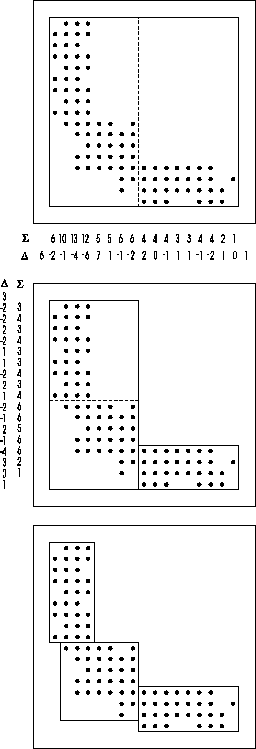
Figure 1: The effect of procedure saw up.
After generation of non-overlapping rectangles in the procedure saw up, it is not guaranteed that all rectangles are properly nested in the rectangles of the parent level. A typical example, where this is not the case, is shown in Figure 2.
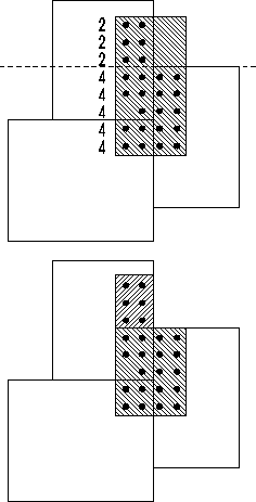
Figure 2: The result of the nesting procedure.
To check, whether a rectangle is properly nested we calculate the sum of areas of intersections with all rectangles of the parent level. When this area equals the area of the actual rectangle it is guaranteed that this rectangle is properly nested. Otherwise, we proceed as follows. First, we determine the longest common edge of the just calculated intersections. Our strategy is to avoid coinciding cuts of several levels. Therefore, we seek for cuts perpendicular to the longest common edge. Let us assume, as in Figure 2, that this edge lies in the y-direction. Then, we cut where the number of grid points covered by the intersections in each row changes. This list of rectangles is recursively tested for proper nesting. Obviously, this procedure is well suited to assign parents to each rectangle at the same time. After having obtained a list of properly nested rectangles, they get information about their neighbors.
In order to extract physical properties of the simulation, it is necessary
to calculate integral quantities like kinetic and magnetic energy as well
as maxima of current density and vorticity. The latter are easily obtained
by looping over all grids and all levels. Integral quantities are calculated
in the following way. First, on the coarsest level the energy ![]() (swiss
cheese energy) associated to the area not covered by grids of higher resolution
is calculated. This is repeated down to the lowest level. Finally, the
energy is obtained as a sum over all energies
(swiss
cheese energy) associated to the area not covered by grids of higher resolution
is calculated. This is repeated down to the lowest level. Finally, the
energy is obtained as a sum over all energies ![]() .
.
On shared memory machines our adaptive mesh refinement code can be parallelized
in an effective and straight forward way. The main time of the program
is spent in the procedure singlestep. Since the number of grids
is much higher than the number of processors parallelization is done by
distributing the grids to the processors. That means that as soon as a
singlestep on a grid is finished, the next grid is passed to the free processor.
This results in a very effective utilization of all processors. All this
can easily be done using standard Posix threads. The implementation on
distributed memory machines using the shared memory access model is in
work.
In contrast to simulations of Frisch et al. [12] and Sulem et al. [11], we choose as initial condition a modified Orszag--Tang vortex, given by
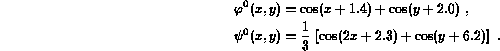
This initial condition, which was already used in turbulence simulations
[13,10],
possesses less symmetry and is therefore more generic for the formation
of small-scale structures. Computations are done with periodic boundary
conditions on a square of length ![]() .
The initial spatial resolution was given by
.
The initial spatial resolution was given by ![]() grid
points.
grid
points.
The temporal evolution of the current density is shown in the color
plots of Figure 3. In addition to the
color levels, the rectangle hierarchy is plotted. The first plot shows
the initial condition and the second the grid after the first refinement
has taken place. The color plot at time t=2.0 contains already
3 levels. At the final time t=2.5 a total of 5 levels are
present. In the actual simulation, the refinement factor was equal to r=2.
On a workstation with 128 Mbyte of main memory, four refinements could
be realized corresponding to a resolution of ![]() grid
points with a non-adaptive scheme. The limiting factor is the amount of
main memory available, whereas up to this resolution computational costs
are very moderate.
grid
points with a non-adaptive scheme. The limiting factor is the amount of
main memory available, whereas up to this resolution computational costs
are very moderate.
time = 0:

time = 1.5:

time = 2.0:

time = 2.5:

In the second picture the current sheets start to form, afterwards they
evolve into thiner and thiner sheets and the maxima of current density
and vorticity are increasing continually. The current density is growing
exponentially in time. In Figure 5 a
semilogarithmic plot of the maximum current density in the upper sheet
is depicted. Included is a fit to an exponential function given by ![]() .
This functional behavior is in agreement with the results of Sulem et
al. [11]. A detailed
analysis of the asymptotic scaling behavior and a comparison to the predictions
in [11] will be presented
elsewhere.
.
This functional behavior is in agreement with the results of Sulem et
al. [11]. A detailed
analysis of the asymptotic scaling behavior and a comparison to the predictions
in [11] will be presented
elsewhere.
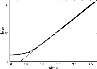
Figure 5: Amplification of current density.
The second order upwind scheme produces substantial energy dissipation only if underresolved steep gradients have formed. Therefore, the energy conservation is a measure whether the singular current sheets are sufficiently resolved. In Figure 6 we give a plot of energy as a function of time. To be more precise, total energy is conserved to within less than 1 %.
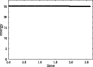
Figure 6: Energy conservation.
In order to further illustrate that the current sheets are well resolved, in Figure 7 we show one dimensional cuts in x-direction through the maximum of current density in the upper half of the integration range. In the upper plot the x-range equals the periodicity length. The lower one with a reduced plot range shows that the grid points of the finest levels very well resolve the current sheet.
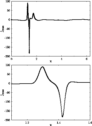
Figure 7: Cuts of current density in x-direction through
the maximum at time ![]() .
.
In the previous section we mentioned that a refinement would take place
when the discretization error for the nonlinearity exceeds a prescribed
value ![]() . The choice
of the parameter
. The choice
of the parameter ![]() is
crucial for the numerical accuracy. If
is
crucial for the numerical accuracy. If ![]() is
taken too large, certain regions may be underresolved which can lead to
reconnection and violation of energy conservation. Decreasing systematically
the value of
is
taken too large, certain regions may be underresolved which can lead to
reconnection and violation of energy conservation. Decreasing systematically
the value of ![]() has
the effect that reconnection phenomena are suppressed. Below a certain
threshold the numerical results proved to be independent of
has
the effect that reconnection phenomena are suppressed. Below a certain
threshold the numerical results proved to be independent of ![]() .
The simulations shown in Figure 3 were
performed with
.
The simulations shown in Figure 3 were
performed with ![]() .
.
Applying adaptive mesh refinement to the evolution of singular structures
like current sheets in magnetohydrodynamics is motivated by the expected
reduction of memory needed to resolve them. This is well justified by the
numerical results. To give the reader an impression of how many grids are
generated on the different levels and of the number of grid points contained
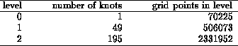
in each level's grids, we display values for the level hierarchy at time
![]() in the following
tables. In Table I the results are shown for a simulation with refinement
factor r=2 and in II for another one with r=4.
in the following
tables. In Table I the results are shown for a simulation with refinement
factor r=2 and in II for another one with r=4.
TABLE I
Statistics for simulation with r = 2.
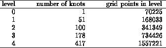
TABLE II
Statistics for simulation with r = 4.
From level to level the total number of grid points grows much less
than by a factor of ![]() necessary
for a non-adaptive treatment. For r chosen equal to 2, one
can see that even for the very small value of
necessary
for a non-adaptive treatment. For r chosen equal to 2, one
can see that even for the very small value of ![]() prescribed
here it increases no more than by a factor of about 2. This promises
that the compression rate will improve the more refinements are performed.
prescribed
here it increases no more than by a factor of about 2. This promises
that the compression rate will improve the more refinements are performed.
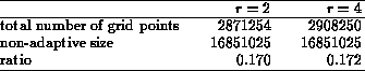
In Table III simulations with different refinement factors are compared with regard to the total number of grid points on all levels. The number of grid points on one data field with the same grid spacing as the finest level in the adaptive code is called the non-adaptive size. In the last row we give the ratio of the grid points, adaptively and non-adaptively. For the investigated hierarchy of 5 levels with refinement factor r=2 this ratio is about 17 %. When the finest levels are equally resolved, the compression for both refinement factors is practically indistinguishable. For the comparison of adaptive versus non-adaptive treatment, the compression rate based on counting grid points does not fully reflect the total improvement in main memory consumption. In upwind schemes several auxiliary fields have to be stored. In non-adaptive simulations these full sized fields are present all the time whereas here they are needed only temporarily during the execution of singlestep on a small grid.
TABLE III
Comparison of different refinement factors.
We want to finish this section with an impressive comparison of the
results for the amplification of the current density for several non-adaptive
grid sizes and for the adaptive code. Figure 8
is a parametric plot of the maximum of current density as a function of
the fit ![]() already
depicted in Figure 5. In addition to
the results of the adaptive mesh refinement code we include data obtained
with fixed grids of resolutions
already
depicted in Figure 5. In addition to
the results of the adaptive mesh refinement code we include data obtained
with fixed grids of resolutions ![]() ,
,
![]() and
and ![]() .
Until the simulations become underresolved, a linear behavior is also observed
in the non-adaptive simulations. Then the upwind method introduces numerical
viscosity leading to reconnection processes and substantial energy dissipation.
.
Until the simulations become underresolved, a linear behavior is also observed
in the non-adaptive simulations. Then the upwind method introduces numerical
viscosity leading to reconnection processes and substantial energy dissipation.
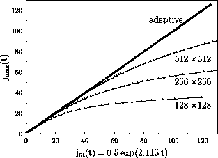
Figure 8: Comparison of adaptive and non-adaptive simulations.
The complexity of adaptive mesh refinement compared to non-adaptive treatments should not be underestimated. On the other hand, the growing progress of object oriented programming languages helps enormously to reduce the difficulties in programming. To give some impression, the programs needed for regridding, nesting and the handling of data structures are only about 3000 lines of C++ code.
As we have demonstrated, adaptive mesh refinement is a powerful tool to study the evolution of singular structures as the formation of current sheets in ideal MHD. Other problems of this type like in the axisymmetric [14] and the full three dimensional Euler equations are natural candidates for this method. Work in this direction is in progress.
Whether adaptive mesh refinement is also a useful concept for simulating turbulent hydro- and magnetohydrodynamic flows will depend on how efficiently the small scale structures can be covered by hierarchically nested grids.
We like to thank K. H. Spatschek for his continuous support. This work was performed under the auspices of the Sonderforschungsbereich 191.
Rainer Grauer
Tue Aug 20 12:21:46 MET DST 1996