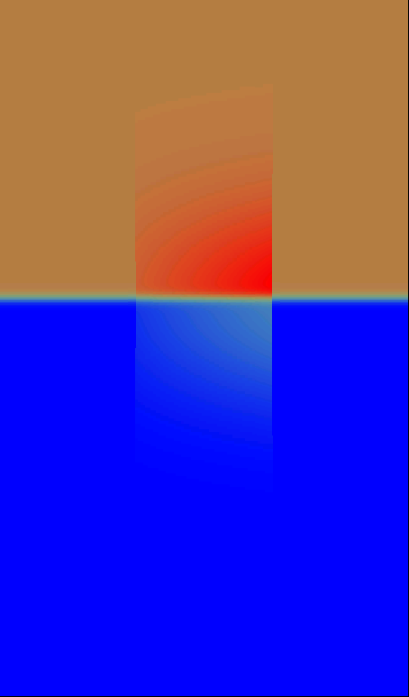
A time-dependent computation based on a Runge-Kutta integrator with a 2-dimensional version of the Kurganov-Levy CWENO scheme simulates the temporal developent of this system. Boundary conditions are periodic in the horizontal direction and no-flow at the bottom and top.
|
|
|
|
|
|
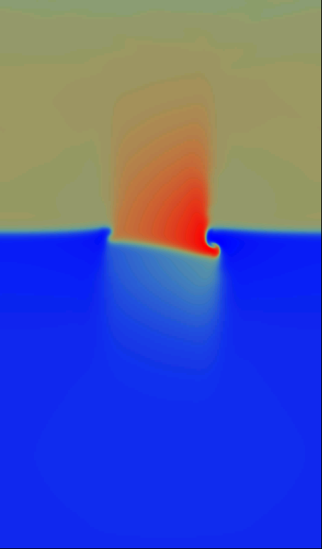
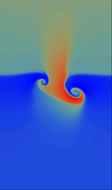
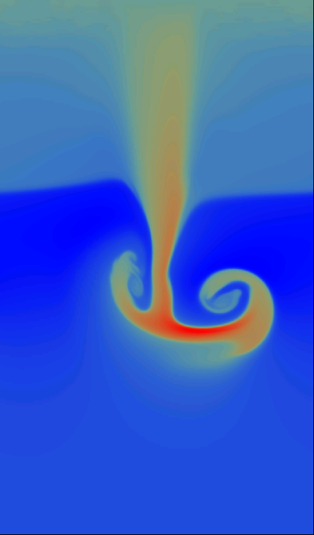
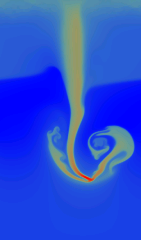
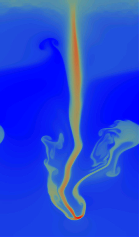
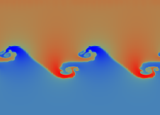
As can be seen from the snapshots, the heavier fluid portions sink downwards and get compressed to even higher density. Note that the colour scaling changes between the pictures: In the base of the downward stream in the very last picture, the density reaches values of 2.75 as compared to peak values of 1.17 in the initial configuration.
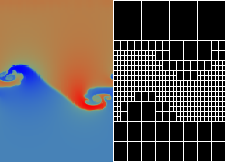
Obviously, the downstreaming fluid creates a turbulent wake, consisting of eddy-like structures that are generated by Kelvin-Helmholtz modes in the shear flow. To resolve these features efficiently, the critical regions of the flow are covered by successively refined meshes, while the less critical regions use coarser, and thereby computaionally cheaper, grids.
Following are the stages of the third, 5th and 6th picture from above, magnified to a 1:1 aspect ratio and with the actual grid coverage superimposed. Each of the subgrids consists of 10 x 16 cells, irrespective of size. In this example, we used a refinement criterion based on the gradient of the mass density. A combination with a flow-based criterion, e.g. the vorticity, might be an interesting alternative?
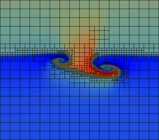
From the upper picture, it becomes clear that only a small fraction of the domain is represented with a high resolution. By far the biggest part is resolved by what amounts to only 160 x 256 grid cells globally, saving quite a lot of computing time. However, the smallest subgrids correspond to a global resolution of 10240 x 16384 cells.
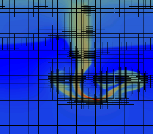
In the second picture, the adaptive aspect of the mesh refinement can be seen very clearly: With the growth and downward motion of the vortex structures and the corresponding formation of density gradients, high resolution meshes are created where necessary (and removed when no more needed). This cluster of refined grids follows the overall evolution.
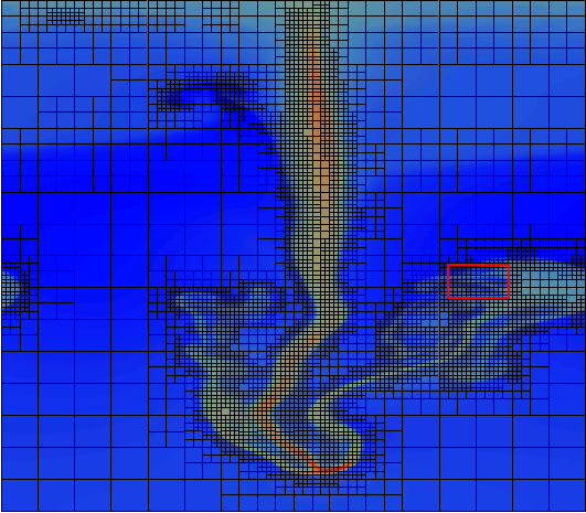
Even in the last picture, where the turbulent region has spread
considerably, only one quarter of the entire domain is covered by grids of the
highest resolution.
As by far the most computation time is needed for the
CWENO-reconstruction and the flux computation, there is still a good
trade-off compared to a simulation with one homogeneous grid - not to
talk about the computation time spent to get here.
At this stage, the domain is covered by 5011 separate grids, 4080 of which
are the smallest "Level 7" grids (You might want to check that I've
counted 'em correctly?).
Also note that, because of the periodic boundary conditions, the structure
re-enters the domain from the left.
An here's a zoom-in of the red rectangle region in the above (with re-scaled colours) -
still resolved with approx. 130 x 100 cells and a 3rd order CWENO scheme.
 |
The temporal evolution of the mass density (colour scale blue to red, file size ca. 1 MByte) |
 |
As above, with the grid coverage of the domain shown. Each grid consist of 16 x 28 cells (file size ca. 1 MByte). |