Mesh Refinement

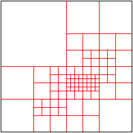
Since the pioneering work of Berger and Colella (J. Comp. Phys., 82, 64, 1989), adaptive mesh refinement (AMR) has become a widespread technique for handling localized structures like shocks etc. on both, structured and unstructured grids. As for structured grids, many of current AMR implementations are based on the original proposal by Berger and Colella to cover critical regions of a coarse grid with patches of finer grids that are "cut" to appropriate size and shape.
Instead of this patch-based refinement, we follow the idea of a strictly regular subgridding: A grid (or block) can only be subdivided into 4 (in 2D) or 8 (in 3D) equally sized subgrids. This refinement, of course, can is recursively until the desired resolution is obtained, or up to a maximum refinement level. The figure to the right demonstrates the principle.

This block-oriented refinement approach is used by a number of other AMR codes as well and makes the data handling much easier than a patch-based refinement: There are well-defined boundaries between neighbouring grids, a refinement always replaces exactly an entire grid with a clear 4-to-1 or 8-to-1 relationship between parents and children.

Often, the created grid hierarchy is kept in a tree-data structure, using pointers to the grid instances. As an alternative approach, racoon II uses a well-defined linear ordering for the grids, based on IDs: Every grid is uniquely identified by two integer numbers - its refinement level and a running ordering number for this particular level. This grid ID alone provides all essential information about a grid, like its (potential) neighbours, children and parent, its position in the domain, the size etc. The ordering itself could be a simple row-by-row numbering, but in order to facilitate an efficient distribution among processors in a distributed environment as described later, we use space filling curves instead.

Also, for distributed simulations, the advantage of a linear ordering becomes evident: Grids can be "addressed" over address space boundaries using their IDs, which allows for a great part of the framework to be programmed without taking care of whether a grid is actually local or remote. In the end, of course, we have to get a hold of a grid - this is done by a reference lookup in a hash based container, and here, we have a tree-based data structure again!

As a rule, all grids in the system have the same number of cells per direction, so that with each refinement level, the spatial resolution increases by a factor of 2 per direction. Accordingly, the smaller grids have to be integrated with smaller time steps in order to meet the CFL condition. In dispersion-free systems, the time step has to be reduced by factor 2 from one level to the next higher one.

An overall integration step is carried out in a recursive manner: First, integrate all grids of some level one step, and pass temporal and spatial interpolations for boundary values to the grids of the next higher (=finer) level. Then, the next level is integrated a number of times, depending on the necessary time step reduction, and finally, data from the higher level is prolonged downwards to the lower level.

After applying this recursive level-wise integration to all levels from the lowest one to the highest represented level, a single step integration is accomplished.

During the computation, a mesh refinement check is performed regularly every few integration steps or so. Refinement is carried out in a two-step procedure, based on a local criterion:

First, all cells in all meshes are inspected for sufficient resolution, based on a criterion that is defined in a class together with the physical problem itself, and flagged if they are found to be "critical".
After this, an algorithm inspects the positions of critical cells within each grid and flags the grid itself and, depending on the location of the critical cells with in the grid, some or all of its neighbours for refinement.

Finally, all grids that are found to need refinement are replaced by their children, or vice versa, if an existing refinement is jugded to be no more needed.

Through this kind of look-ahead mechanism, refinement of grids can be triggered already before critical structures have entered it. This, of course, has to work independently of whether the neighbour meshes reside in the same process or somewhere else...