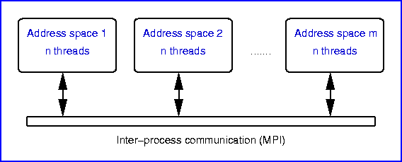
As for the multithreading, we use standard POSIX thread techniques,
where the number of threads to create is a configurable simulation
parameter.
By now, the only tasks that are executed concurrently are the
numerical integration routines, as these are the most critical ones in
terms of runtime, and the exchange of boundary values within one
level.
Diagnostics, output and grid refinement are processed within one
thread. This also applies to the MPI communication as the present
freely available implementations of MPI are not thread safe.
Typical values of the execution time speed-up obtained by
multithreading on one node of the UKMHD cluster (4
DEC Alpha CPUs) are given in the table below. The actual values depend
somewhat on the frequency of data output, refinement checks etc.
| #CPUs | rel. speedup | rel. speedup / #CPUs |
| 1 | 1. | 1. |
| 2 | 1.85 | 0.93 |
| 3 | 2.59 | 0.86 |
| 4 | 3.02 | 0.75 |
In a distributed simulation, data exchanged between grids must
potentially be sent to a different process. Likewise, a global
strategy for the load balancing, i.e. the efficient distribution of
grids among the involved processes, is necessary.
In order to keep a clean separation between the communication aspects
and the rest of the simulation tasks, we defined a transport interface
through which all communication and synchronization is achieved.
One implementation of this interface is based on the Message Passing
Interface (MPI); a second one is an empty null-implementation that we
use in the case of single-process runs; a third one for optimal network
bandwidth exploitation with multi-thread safe MPI implementations is
envisaged.
Load balancing among the processes is realized on the basis of a space filling curve ordering of the grids. Two aspects are vital for reasonable runtime performance of a distributed computation:
In order to keep the communication small, the strategy is to try to
keep clusters of neighbouring grids on the same processor and reduce
the unavoidable remote communication to the borders between such
clusters.
In other words, we try to map the physical neighbourhood of
grids to the neighbourhood in a linear order of the grids - this is
achieved by the use of space filling curves.
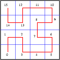 |
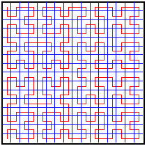 |
In the figures above, 2-dimensional Hilbert curves of levels 2 and 4, respectively, are shown. These curves exists in n dimensions and algorithms are available to map between discrete physical points in an n-dimensional cube and coordinate points on a level l Hilbert curve in this cube. As can be guessed from the pictures and estimated (e.g. Zumbusch, Z. Angew. Math. Mech., 81:25-28, 2001), space filling curves like the Hilbert curves offer the desired property of good neighbourhood conversation.
The strategy for distribution and load balancing is then to order the existing grids of a certain level along the corresponding Hilbert curve and to cut this order into equal pieces, according to the number of processors.
Things get more involved when considering the relationship between different refinement levels: Even here, the neighbourhood can be conserved by ordering all grids in a way where each single grid of a certain level is followed immediately by its children (Zumbusch, 2001). This ordering, that we call the global ordering, assures that communication even between levels tends to be localized. However, it must be taken into account that the integration scheme introduces a temporal separation in that only one refinement level is integrated at a time with synchronization points in between. As a consequence, even though the spatial distribution of the global ordering is close to optimal in that neighbourhood is conserved globally, situations may occur where individual processors idle for entire level integration cycles, simply because they have no grids of the actual integrated level - this would mean a poor load balance!
Both, a global balancer based on a cost function c(l) for a grid of level l and a level-based balancer are implemented in racoon II. Which of these gives the better overall performance depends on the actual arrangement of the grids, in particular the clustering and position of the highest refinement level grids. As these factors change in the course of the simulation, it is hardly possible to make a general statement of which strategy is preferred.
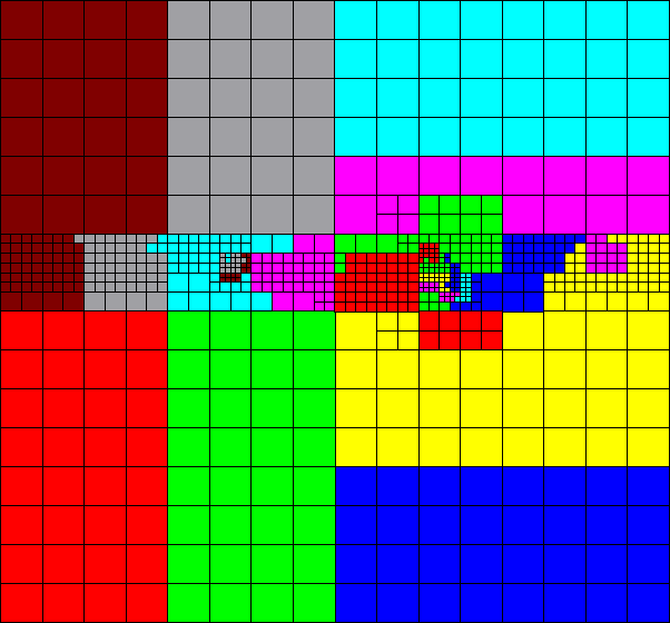
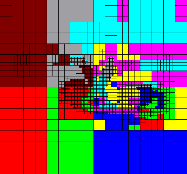
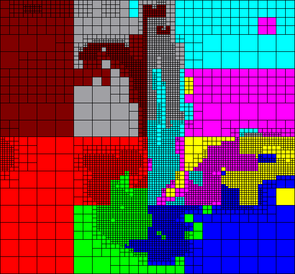
Below are snapshots taken from the example described earlier. The simulation run
was carried out on 8 processors with a per-level balancing, and the
colour code in the pictures indicates which processor each individual
grid resided on at a particular time.
 |
 |
 |
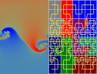 An other example is this movie (1.4 Mbyte file size!):
In the left half, the mass desity is shown as a colour code.
The right side indicates the grid layout, the grid distribution among the 8 processors
(colour code) and the total order of the grids, induced by the space filling curves.
An other example is this movie (1.4 Mbyte file size!):
In the left half, the mass desity is shown as a colour code.
The right side indicates the grid layout, the grid distribution among the 8 processors
(colour code) and the total order of the grids, induced by the space filling curves.
It becomes obvious, why the load balancing is called dynamic!
Load balancing in racoon II is combined with the grid refinement:
Operating a complex simulation in a concurrent and distributed environment poses more challenges than a simple sequentially executing program. As the interaction between the grids across threads and address spaces opens the door for race conditions, failures and deadlocks, often manifesting themselves in strange symptoms, we have equipped the data managing parts of racoon II with additional security measures. For example, guarding flags on each grid keep track of the reception and consumption of boundary values, interpolations etc. to ensure that grids are in a consistent state during the simulation. These relatively simple measures proved to be invaluable to track down subtle programming errors and other problems.